Octave Tutorials by Andrew Ng
Updated at: March 11, 2017
part1: basic
numeric
- five add six,
5+6 - three minus two,
3-2 - five multiplied by eight/five times eight,
5*8 - one divided by two/two into one goes,
1/2 - x to the yth power,
x^y
logic
1 == 2 % false, % is comment1 ~= 0 % not equal to1 && 0 % AND1 || 0 % ORxor(1,0) % 异或
PS1(cmd promot): PS1('>> ');
>> a=3
a =  3
>> a=3; %semicolon suppress output
>> b='hi';
>> c=(3>=1);
>> c
c =  1
>> a=pi;
>> a
a =  3.1416
>> disp(a)
3.1416
>> disp(sprintf('2 decimals: %0.2f',a))
2 decimals: 3.14
>> format long
>> a
a =  3.14159265358979
>> format short
>> a
a =  3.1416
matrix & vector
>> A=[1 2;3 4;5 6]
A =

   1   2
   3   4
   5   6

>> A=[1 2;
3 4;
5 6]
A =

   1   2
   3   4
   5   6

>> v=[1 2 3]
v =

   1   2   3

>> v=[1;2;3]
v =

   1
   2
   3

>> v=1:0.1:2 % start:increment:end
v =

    1.0000    1.1000    1.2000    1.3000    1.4000    1.5000    1.6000    1.7000    1.8000    1.9000    2.0000

>> v=1:6
v =

   1   2   3   4   5   6

>> ones(2,3)
ans =

   1   1   1
   1   1   1

>> C=2\*ones(2,3)
C =

   2   2   2
   2   2   2

>> w = zeros(1,3) % one by three matrix
w =

   0   0   0

>> w=rand(1,3)
w =

   0.37811   0.72512   0.89963

>> rand(3,3) % uniform distribution
ans =

   0.850304   0.011820   0.684585
   0.109987   0.530488   0.862454
   0.155507   0.301278   0.619777

>> randn(3,3) % gauls distribution 正态分布
>> eye(4)
ans =

Diagonal Matrix

   1   0   0   0
   0   1   0   0
   0   0   1   0
   0   0   0   1
>> help eye
figure
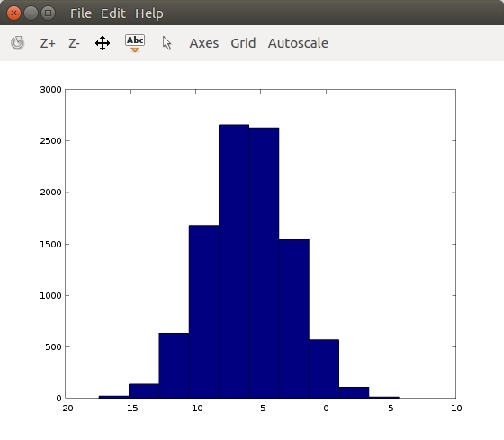
>> w=-6+sqrt(10)\*(randn(1,10000));
>> hist(w)
part2: move data around
>> A=[1 2;3 4;5 6;]
A =

   1   2
   3   4
   5   6

>> size(A)
ans =

   3   2

>> size(A,1) % row count
ans =  3
>> size(A,2) % column count
ans =  2
>> v=[1 2 3 4]
v =

   1   2   3   4

>> length(v)
ans =  4
>> length(A)
ans =  3
>> pwd
ans = /home/xxx
>> cd octave/
>> ls
featuresX.dat  featuresY.dat
>> load featuresX.dat
>> who
Variables in the current scope:

A          ans        featuresX  v

>> featuresX
featuresX =

   1234      1
   4567      2
   1234      3
   4567      4

>> whos
Variables in the current scope:

   Attr Name           Size                     Bytes  Class
   ==== ====           ====                     =====  =====
        A              3x2                         48  double
        ans            1x11                        11  char
        featuresX      4x2                         64  double
        v              1x4                         32  double

Total is 29 elements using 155 bytes
>> load featuresY.dat
>> clear featuresX
>> whos
Variables in the current scope:

   Attr Name           Size                     Bytes  Class
   ==== ====           ====                     =====  =====
        A              3x2                         48  double
        ans            1x11                        11  char
        featuresY      4x1                         32  double
        v              1x4                         32  double

Total is 25 elements using 123 bytes
>> v=featuresY(1:2)
v =

   1234
   4567
>> save hello.mat v;
>> clear
>> load hello.mat
>> who
Variables in the current scope:

v
>> save hello.txt v -ascii % save as text(ASCII)
>> A=[1 2;3 4;5 6]
A =

   1   2
   3   4
   5   6

>> A(3,2)
ans =  6
>> A(3,:) % ":" means every element along that row/col
ans =

   5   6

>> A(:,2)
ans =

   2
   4
   6

>> A([1 3],:)
ans =

   1   2
   5   6
>> A(:,2)=[10;11;12]
A =

    1   10
    3   11
    5   12
>> A=[A,[100;101;102]] % append another column vector to right
A =

     1    10   100
     3    11   101
     5    12   102
>> B=[1 2 3;4 5 6;7 8 9]
B =

   1   2   3
   4   5   6
   7   8   9

>> C=[A B]
C =

     1    10   100     1     2     3
     3    11   101     4     5     6
     5    12   102     7     8     9
>> C=[A;B]
C =

     1    10   100
     3    11   101
     5    12   102
     1     2     3
     4     5     6
     7     8     9
part3: compute on data
>> A=[1 2;3 4;5 6]
A =

   1   2
   3   4
   5   6

>> B=[11 12;13 14;15 16]
B =

   11   12
   13   14
   15   16

>> C=[1 1;2 2]
C =

   1   1
   2   2

>> A*C
ans =

    5    5
   11   11
   17   17
>> A.*B
ans =

   11   24
   39   56
   75   96
>> A.^2
ans =

    1    4
    9   16
   25   36
>> v=[1;2;3]
v =

   1
   2
   3

>> 1./v
ans =

   1.00000
   0.50000
   0.33333
>> log(v)
ans =

   0.00000
   0.69315
   1.09861

>> exp(v)
ans =

    2.7183
    7.3891
   20.0855
>> abs([-1;-2;-3])
ans =

   1
   2
   3
>> -v % -1*v
ans =

  -1
  -2
  -3
>> v+ones(length(v),1)
ans =

   2
   3
   4
>> A' % ' meas transpose
ans =

   1   3   5
   2   4   6
>> (A')'
ans =

   1   2
   3   4
   5   6
>> value=max(v)
value =  3
>> [value,index]=max(v)
value =  3
index =  3
>> v<2
ans =

   1
   0
   0
>> [row,col]=find(A>=7)
row =

   1
   3
   2

col =

   1
   2
   3
>> a=[1.000 15.000 2.000 0.500]
a =

    1.00000   15.00000    2.00000    0.50000

>> sum(a)
ans =  18.500
>> prod(a) % multiply
ans =  15
>> floor(a)
ans =

    1   15    2    0
>> ceil(a)
ans =

    1   15    2    1
>> max(rand(3),rand(3)) % For two matrices (or a matrix and a scalar), return the pairwise maximum.
ans =

   0.86233   0.98616   0.82504
   0.82724   0.70070   0.31207
   0.89491   0.58022   0.97937
>> max(A,[],1)
ans =

   8   9   7

>> max(A,[],2)
ans =

   8
   7
   9
>> max(A)
ans =

   8   9   7

>> max(max(A))
ans =  9
>> max(A(:))
ans =  9
>> A=magic(9)
A =

   47   58   69   80    1   12   23   34   45
   57   68   79    9   11   22   33   44   46
   67   78    8   10   21   32   43   54   56
   77    7   18   20   31   42   53   55   66
    6   17   19   30   41   52   63   65   76
   16   27   29   40   51   62   64   75    5
   26   28   39   50   61   72   74    4   15
   36   38   49   60   71   73    3   14   25
   37   48   59   70   81    2   13   24   35

>> sum(A,1)
ans =

   369   369   369   369   369   369   369   369   369

>> sum(A,2)
ans =

   369
   369
   369
   369
   369
   369
   369
   369
   369
>> A .* eye(9)
ans =

   47    0    0    0    0    0    0    0    0
    0   68    0    0    0    0    0    0    0
    0    0    8    0    0    0    0    0    0
    0    0    0   20    0    0    0    0    0
    0    0    0    0   41    0    0    0    0
    0    0    0    0    0   62    0    0    0
    0    0    0    0    0    0   74    0    0
    0    0    0    0    0    0    0   14    0
    0    0    0    0    0    0    0    0   35
>> sum(sum(A .* eye(9)))
ans =  369
>> flipud(eye(9))
ans =

Permutation Matrix

   0   0   0   0   0   0   0   0   1
   0   0   0   0   0   0   0   1   0
   0   0   0   0   0   0   1   0   0
   0   0   0   0   0   1   0   0   0
   0   0   0   0   1   0   0   0   0
   0   0   0   1   0   0   0   0   0
   0   0   1   0   0   0   0   0   0
   0   1   0   0   0   0   0   0   0
   1   0   0   0   0   0   0   0   0
>> A=magic(3)
A =

   8   1   6
   3   5   7
   4   9   2

>> pinv(A) % pseudoinverse of X 广义逆矩阵(伪逆矩阵)
ans =

   0.147222  -0.144444   0.063889
  -0.061111   0.022222   0.105556
  -0.019444   0.188889  -0.102778

>> pinv(A) * A
ans =

   1.0000e+00   2.0817e-16  -3.1641e-15
  -6.1062e-15   1.0000e+00   6.2450e-15
   3.0531e-15   4.1633e-17   1.0000e+00
part4: plot data
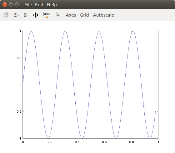
>> t=[0:0.01:0.98];
>> y1=sin(2*pi*4*t);
>> plot(t,y1);
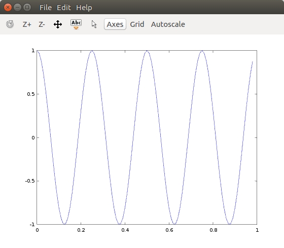
>> y2=cos(2*pi*4*t);
>> plot(t,y2)
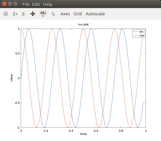
>> plot(t,y1);
>> hold on;
>> plot(t,y2,'r');
>> xlabel('time')
>> ylabel('value')
>> legend('sin','cos')
>> title('my plot')
>>
>> print -dpng 'myplot.png'
>> figure(1); plot(t,y1);
>> figure(2); plot(t,y2); % two figure windows
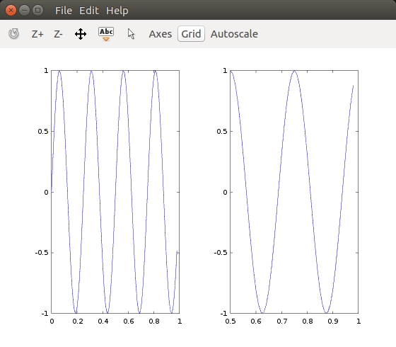
>> subplot(1,2,1) % divides plota 1x2 grid, access first element
>> plot(t,y1);
>> subplot(1,2,2);
>> plot(t,y2);
>> axis([0.5 1 -1 1])
>> clf; % clean plot
>> A=magic(5)
A =

   17   24    1    8   15
   23    5    7   14   16
    4    6   13   20   22
   10   12   19   21    3
   11   18   25    2    9

>> imagesc(A)
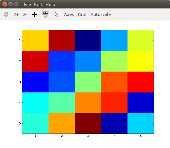
>> imagesc(A)
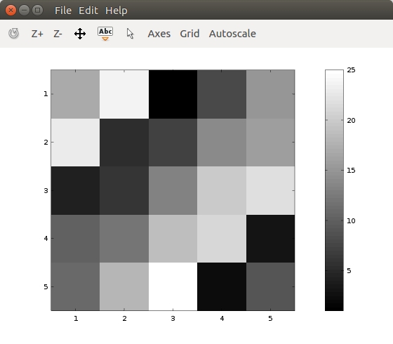
>> imagesc(A), colorbar, colormap gray;
part5: control statement
>> v=zeros(10,1);
>> for i=1:10,
v(i)=2^i;
end;
>> v
v =

      2
      4
      8
     16
     32
     64
    128
    256
    512
   1024
>> indices=1:10;
>> for i=indices,
disp(i);
end;
 1
 2
 3
 4
 5
 6
 7
 8
 9
 10
>> i=1;
>> while i<=5,
v(i)=100;
i=i+1;
end;
>> v
v =

    100
    100
    100
    100
    100
     64
    128
    256
    512
   1024
>> i=1;
>> while true,
    v(i)=999;
    i=i+1;
    if i==6,
      break;
    end;
   end;
>> v
v =

    999
    999
    999
    999
    999
     64
    128
    256
    512
   1024
>> v(1)=2;
>> if v(1)==2,
     disp('v(1) is two');
   elseif v(1)==1,
     disp('v(1) is one');
   else
     disp('v(1) is not one or two');
   end;
v(1) is two
function
%squareThisNumber.m
function y = squareThisNumber(x)

y = x^2;
%%%%%%%%%%%%%%%

>> squareThisNumber(5)
ans =  25
>> squareThisNumber(5)
ans =  25
>> % Octave search path
>> addpath('someplace')

%squareAndCubeThisNumber.m
function [y1,y2] = squareAndCubeThisNumber(x)

y1 = x^2
y2 = x^3
%%%%%%%%%%%%%%%

>> [a,b]=squareAndCubeThisNumber(2)
y1 =  4
y2 =  8
a =  4
b =  8
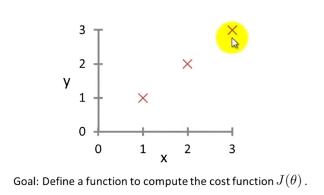
%costFunctionJ.m
function J = costFunctionJ(X, y, theta)

% X is the "design matrix" containing our training examples
% y is the class labels

m = size(X, 1); % number of training examples
predictions = X*theta; % predictions of hypothesis on all m examples
sqrErrors = (predictions - y).^2; % squared errors

J = 1/(2*m) * sum(sqrErrors);
%%%%%%%%%%%%%%%%

>> X=[1 1;1 2;1 3];
>> y=[1;2;3];
>> theta=[0;1];
>> j=costFunctionJ(X,y,theta)
j = 0
>> theta=[0;0];
>> j=costFunctionJ(X,y,theta)
j =  2.3333
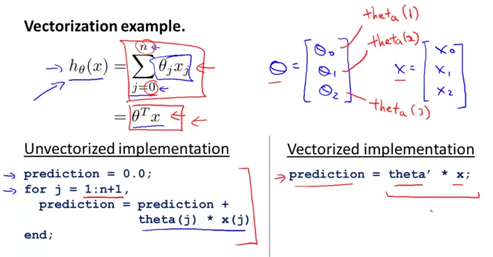
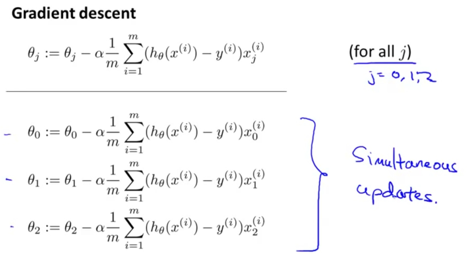
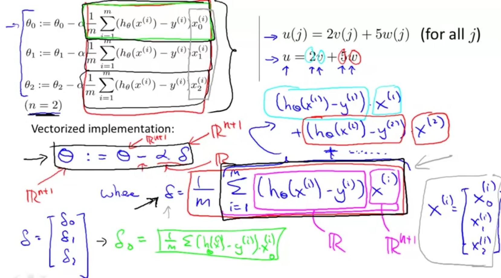
part6: Vectorization